This web page was produced as an assignment for an undergraduate course at Davidson College.
“The complete genome sequence of Lactobacillus bulgaricus reveals extensive and ongoing reductive evolution”. The title is the first thing in the paper and it’s the first thing I appreciate about it. It is direct, it is complete, and it is immediately interesting. I do wish the authors might say “suggests” instead of “reveals”, for the dual reasons that I don’t think the more cautious term detracts significantly from the effect, and that the more doubt the authors inject into the paper, the more likely I am to be open to their claims.
This is my only critique of the article, and it is relatively small—that the authors didn’t fully enough entertain alternatives to their theory of reductive evolution. Their theory might be watertight as anything, but they ought at least to give some weight to other ideas that might sink their theory; then they can go ahead and prove those ideas untenable. They mentioned alternate interpretations of their data in most cases, but didn’t provide much analysis of them, so it seemed like the authors might have been a little bit blinded by the obvious connection they made between specialized/reductive evolution and the position of the L. bulgaricus genome. I would have liked them to consider more fully the possibility that their conclusions were wrong, and then to revisit their data and find possible alternate explanations for their observations.
That said, I am convinced. The authors really do a very clear job presenting their theory that the genome of L. bulgaricus is undergoing reductive evolution. This reductive evolution is a result of ongoing specialization for a specific environment, they argue, and give four major supporting points of evidence. First, there are an unusually high number of pseudogenes and incomplete metabolic pathways. Second, there are an unusually high number of RNA genes. Third, the GC3 content is unusually high. Fourth, the lengthy inverted repeat near the replication terminus is unusual. These factors are all unusual for a typical bacterial genome, the authors argue, but are to be expected if the genome were undergoing reductive evolution; therefore the simplest explanation is that the genome must be undergoing reductive evolution.
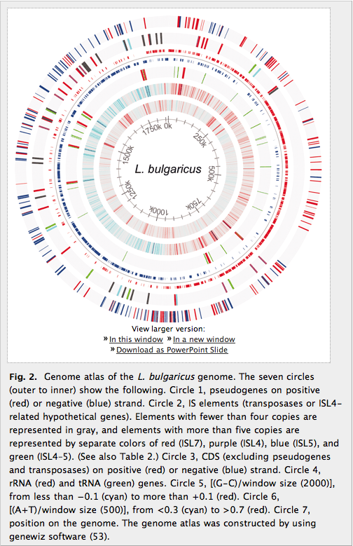
Figure 1: GC3 content is unusually high
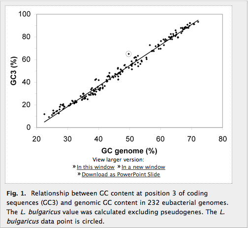
Figure 1 is simple and easy to read. It shows the GC3 content as related to the genomic GC content for various genomes. The points clearly follow a direct relationship and the line of best fit is plotted; the point for the L. bulgaricus genome (circled) stands out as one of the outliers from the regression because its GC3 content is unusually high compared to its genomic GC content. The point is easy to see, but I’m not convinced of how significant the difference is. Ours is probably the clearest outlier on the graph, but I wonder if a p-value could be calculated to determine how likely it is that the point is a statistical outlier. I also wonder if pseudogenes were excluded from the other 232 calculations (as they were in our genome), and if not, would excluding them still leave L. bulgaricus an outlier? These points ought to be addressed to offer a truly convincing argument.
Figure 2: The L. Bulgaricus genome
Figure 2 is visually very busy and it’s difficult to follow at first glance. It proves to be very informative, however, once the colors and layers are decoded. We’ll analyze it from the outside in. (1) The outermost circle shows the surprising number of pseudogenes—there are a lot. This is subjective rather than objective, and I don’t think it would be at all useful to try to fit an objective comparison to other genomes in this figure, but I wish the authors would address this in the text when they note that 270 is a high number for pseudogenes. This layer also shows each pseudogene’s position on either the positive or negative strand, a coloring scheme that is followed in the other layers of the circle unless noted otherwise. (2) The next circle shows insertion sequence elements, and the principal noteworthy feature here is the complete absence of any IS elements between 279 kbp and 694 kbp. (3) Circle three shows the coding sequences and their positions on the positive (red) or negative (blue) strands. One can easily see where the replication origin and terminus are located based on the areas where the greatest concentration of genes switches from being on the positive strand to the negative strand. (4) This circle shows the locations of rRNA and tRNA genes. (5) and (6). I’m not sure what these circles represent—GC skew is my impression, but I don’t know what (G-C) is in comparison to (A+T) and it’s not defined in the paper. Circle 5 is at the macro level with a relatively large sliding window size, and one can see pretty clearly where the replication origin and terminus are, while circle 6 shows the micro level better with a smaller sliding window size. (7) The innermost circle shows position in kbp on the genome.
Figure 3: RNA genes related to genome size
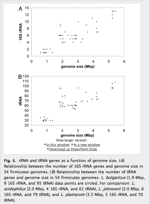
Figure 3 is a two-part figure showing the relation between the number of 16S rRNA genes (part A) or tRNA genes (part B) and genome size. This is a direct relationship, so as genome size increases the number of RNA genes tends also to increase. 55 different points represent L. bulgaricus and 54 related genomes; L. bulgaricus, as in Figure 1, is clearly an outlier, with more RNA genes than one would expect based on its genome size. I like the description in the text of the relation between the average numbers and those in L. bulgaricus, and I like the alternate explanation given that rRNA and tRNA gene counts might vary according to capacity to survive in different environments.
Figure 4: Synteny between L. bulgaricus and L. acidophilus
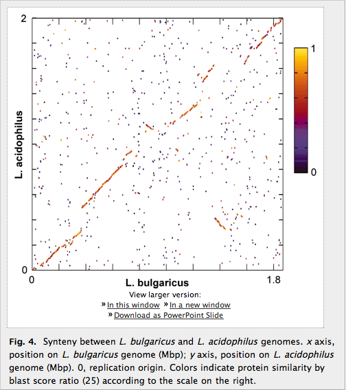
Figure 4 shows the two genomes of L. bulgaricus and L. acidophilus on the x- and y-axis, respectively, and genes are colored according to BLAST protein similarity. Synteny is widespread, as shown by the left-to-right ascending diagonal line. There are three regions of perturbation: two about 400kbp from the origin in either direction (closer to the left and right sides of the figure), and one large one around the replication terminus (in the middle of the figure). The figure highlights the “backbone” of similarity between the two genomes, and also the regions of difference that constitute mostly unknown functions, as well as some differences in completeness of pathways.